Traditional power system, system setup
Contents
Traditional power system, system setup#
Here we present the creation of a small example network in RELSAD. The network consists of 6 buses and 6 lines, where one of the lines is a backup line. We introduce simplified loads.
Imports#
To create a power system the necessary imports need to be added.
We will make use of os, numpy, pandas and matplotlib in this tutorial:
import os
import numpy as np
import pandas as pd
import matplotlib.pyplot as plt
For importing components from RELSAD:
from relsad.network.components import (
    Bus,
    Line,
    Disconnector,
    CircuitBreaker,
    ManualMainController,
)
For importing systems and networks from RELSAD:
from relsad.network.systems import (
    PowerSystem,
    Transmission,
    Distribution,
)
To run time dependent simulations, the time utilities of RELSAD must be imported:
from relsad.Time import (
    Time,
    TimeUnit,
    TimeStamp,
)
Adding statistical distribution for, for example, outage time of components, is done by using the statistical distribution utilities of RELSAD, which needs to be imported:
from relsad.StatDist import (
    StatDist,
    StatDistType,
    NormalParameters,
)
The statistical distribution utilities of RELSAD enables a variety of custom distributions, including normal and uniform distributions.
To prioritize the bus loadings during outages, the user may define cost functions that can be related to chosen buses. To use this feature, the CostFunction class must be imported:
from relsad.load.bus import CostFunction
To plot the network topology, we import the plot_topology function:
from relsad.visualization.plotting import plot_topology
The Simulation class must be imported to be able to run simulations:
from relsad.simulation import Simulation
Create components#
First, we create the components for our system.
Creating buses:
# Failure rate and outage time of the transformer on the bus
# are not necessary to add, this can be added on each bus.
# Their default values are 0 and Time(0) respectively.

B1 = Bus(
    name="B1",
    n_customers=0,
    coordinate=[0, 0],
)
B2 = Bus(
    name="B2",
    n_customers=1,
    coordinate=[1, 0],
)

B3 = Bus(
    name="B3",
    n_customers=1,
    coordinate=[2, 1],
)

B4 = Bus(
    name="B4",
    n_customers=1,
    coordinate=[2, 0],
)

B5 = Bus(
    name="B5",
    n_customers=1,
    coordinate=[3, 0],
)

B6 = Bus(
    name="B6",
    n_customers=1,
    coordinate=[3, 1],
)
Creating lines:
# Failure rate and outage time of the lines can be added to each line.
# The default value of the line failure rate is 0, while the default
# outage time is 0 (Uniform float distribution with max/min values of 0).

# For adding statistical distributions, in this case a
# truncated normal distribution:

line_stat_repair_time_dist = StatDist(
    stat_dist_type=StatDistType.TRUNCNORMAL,
    parameters=NormalParameters(
        loc=1.25,
        scale=1,
        min_val=0.5,
        max_val=2,
    ),
)

fail_rate_line = 0.07

L1 = Line(
    name="L1",
    fbus=B1,
    tbus=B2,
    r=0.5,
    x=0.5,
    fail_rate_density_per_year=fail_rate_line,
    repair_time_dist=line_stat_repair_time_dist,
)
L2 = Line(
    name="L2",
    fbus=B2,
    tbus=B3,
    r=0.5,
    x=0.5,
    fail_rate_density_per_year=fail_rate_line,
    repair_time_dist=line_stat_repair_time_dist,
)
L3 = Line(
    name="L3",
    fbus=B2,
    tbus=B4,
    r=0.5,
    x=0.5,
    fail_rate_density_per_year=fail_rate_line,
    repair_time_dist=line_stat_repair_time_dist,
)
L4 = Line(
    name="L4",
    fbus=B4,
    tbus=B5,
    r=0.5,
    x=0.5,
    fail_rate_density_per_year=fail_rate_line,
    repair_time_dist=line_stat_repair_time_dist,
)
L5 = Line(
    name="L5",
    fbus=B3,
    tbus=B6,
    r=0.5,
    x=0.5,
    fail_rate_density_per_year=fail_rate_line,
    repair_time_dist=line_stat_repair_time_dist,
)

# Backup line

L6 = Line(
    name="L6",
    fbus=B4,
    tbus=B6,
    r=0.5,
    x=0.5,
    fail_rate_density_per_year=fail_rate_line,
    repair_time_dist=line_stat_repair_time_dist,
)

# Set L6 as a backup line

L6.set_backup()
Creating circuit breaker:
E1 = CircuitBreaker(
    name="E1",
    line=L1,
)
Creating disconnectors:
Disconnectors can be added to the lines in the system. A line can have zero, one or two disconnectors connected. In this example, we add several disconnectors for each line. If a circuit breaker is placed on a line, can also have two disconnectors:
DL1a = Disconnector(
    name="L1a",
    line=L1,
    bus=B1,
)
DL1b = Disconnector(
    name="L1b",
    line=L1,
    bus=B2,
)
DL2a = Disconnector(
    name="L2a",
    line=L2,
    bus=B2,
)
DL2b = Disconnector(
    name="L2b",
    line=L2,
    bus=B3,
)
DL3a = Disconnector(
    name="L3a",
    line=L3,
    bus=B2,
)
DL3b = Disconnector(
    name="L3b",
    line=L3,
    bus=B4,
)
DL4a = Disconnector(
    name="L4a",
    line=L4,
    bus=B4,
)
DL4b = Disconnector(
    name="L4b",
    line=L4,
    bus=B5,
)
DL5a = Disconnector(
    name="L5a",
    line=L5,
    bus=B3,
)
DL5b = Disconnector(
    name="L5b",
    line=L5,
    bus=B6,
)

# For backup line
DL6a = Disconnector(
    name="L6a",
    line=L6,
    bus=B4,
)
DL6b = Disconnector(
    name="L6b",
    line=L6,
    bus=B6,
)
Initialize power system#
For systems without ICT, a manual main controller is added with a name and a desired sectional time:
C1 = ManualMainController(name="C1", sectioning_time=Time(0))
Then the power system is created:
ps = PowerSystem(controller=C1)
Create networks#
After creating the components in the network, the components need to be added to their associated networks and the associated networks must be added to the power system. First, the bus connecting to the overlying network (often transmission network) is added. In this case the overlying network is a transmission network, which is created by:
tn = Transmission(
    parent_network=ps,
    trafo_bus=B1,
)
The distribution network contains the rest of the components, and links to the transmission network with line L1. This is done by the following code snippet:
dn = Distribution(
    parent_network=tn,
    connected_line=L1,
)
dn.add_buses([B2, B3, B4, B5, B6])
dn.add_lines([L2, L3, L4, L5, L6])
Visualize topology#
To validate the network topology, it can be plotted in the following way:
fig = plot_topology(
    buses=ps.buses,
    lines=ps.lines,
    bus_text=True,
    line_text=True,
)

fig.savefig(
    "test_network.png",
    dpi=600,
)
The plot should look like this:
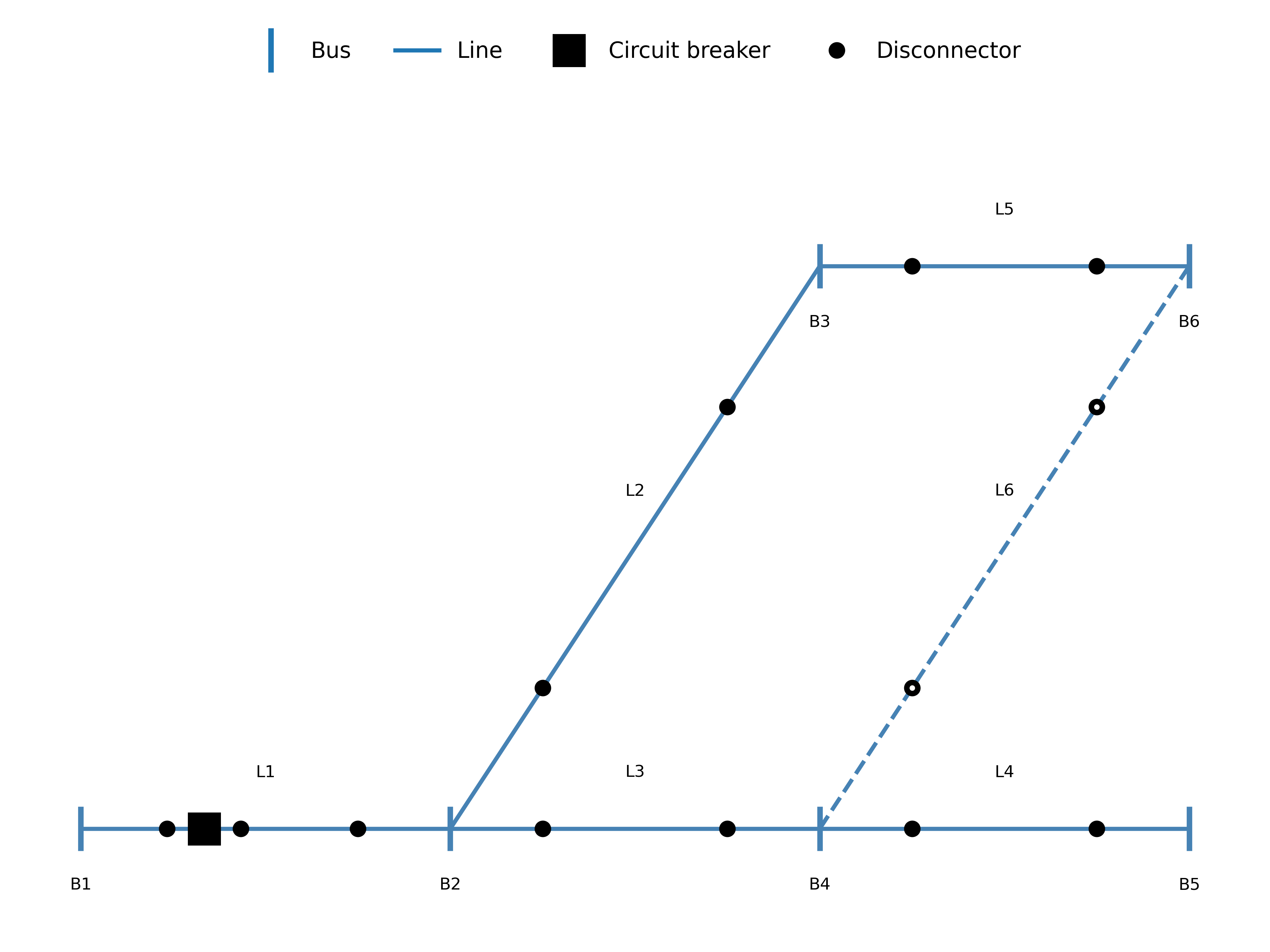
Fig. 1 Test network#
Load and generation#
In Load and generation preparation, examples of how to generate load and generation profiles are provided. The generated profiles can be used to set the load and generation on the buses in the system. The load and generation profiles can then be added to the buses in the system.
For illustration purposes, we defines some constant loads in this tutorial:
load_household = np.ones(365 * 24) * 0.05 # MW
We refer to the example simulations for more realistic load handling.
In addition, a cost related to the load can be added to the bus. For generating the specific interruption cost for a load category:
household = CostFunction(
    A=8.8,
    B=14.7,
)
Load and cost can be added to the buses:
B2.add_load_data(
    pload_data=load_household,
    cost_function=household,
)

B3.add_load_data(
    pload_data=load_household,
    cost_function=household,
)