Traditional power system, Sequential

Here we present how to run a small sequential simulation of the behavior of the network presented in the system setup section to illustrate how RELSAD can be used.

Sequential simulation

To run a sequential simulation the user must specify:

• Simulation start time, start_time

• Simulation stop time, stop_time

• Time step, time_step

• Time unit presented in results, time_unit

• A callback function, callback

• Saving directory for results, save_dir

def callback(ps, prev_time, curr_time):
    dt = curr_time - prev_time
    if curr_time <= dt:
        ps.get_comp("L2").fail(dt=dt)
        ps.get_comp("L6").fail(dt=dt)
    elif Time(1.95, unit=dt.unit) < curr_time < Time(2.05, unit=dt.unit):
        ps.get_comp("L3").fail(dt=dt)


sim = Simulation(power_system=ps, random_seed=0)
sim.run_sequential(
    start_time=TimeStamp(
        year=2019,
        month=0,
        day=0,
        hour=0,
        minute=0,
        second=0,
    ),
    stop_time=TimeStamp(
        year=2019,
        month=0,
        day=0,
        hour=10,
        minute=0,
        second=0,
    ),
    time_step=Time(0.1, TimeUnit.HOUR),
    time_unit=TimeUnit.HOUR,
    callback=callback,
    save_dir="results",
)

Here we used the callback function to specify that line L2 and L6 will fail at the start of the simulation, while line L3 will fail after two hours. The callback function enables easy customization and implementation of scenarios of interest.

To run a deterministic sequential simulation the user must set all failure rates to zero and all repair times to constant values. Otherwise, the simulation will exhibit a stochastic behavior.

Here we plot ENS (Energy Not Supplied) for the power system:

path = os.path.join(
    "results",
    "sequence",
    "ps1",
    "ENS.csv",
)

df = pd.read_csv(path)
fig, ax = plt.subplots()
df.plot(
    x="HOUR",
    y="ps1",
    ax=ax,
)

fig.savefig(
    "ENS.png",
    dpi=600,
)

print(df.describe())

The plot should look like this:

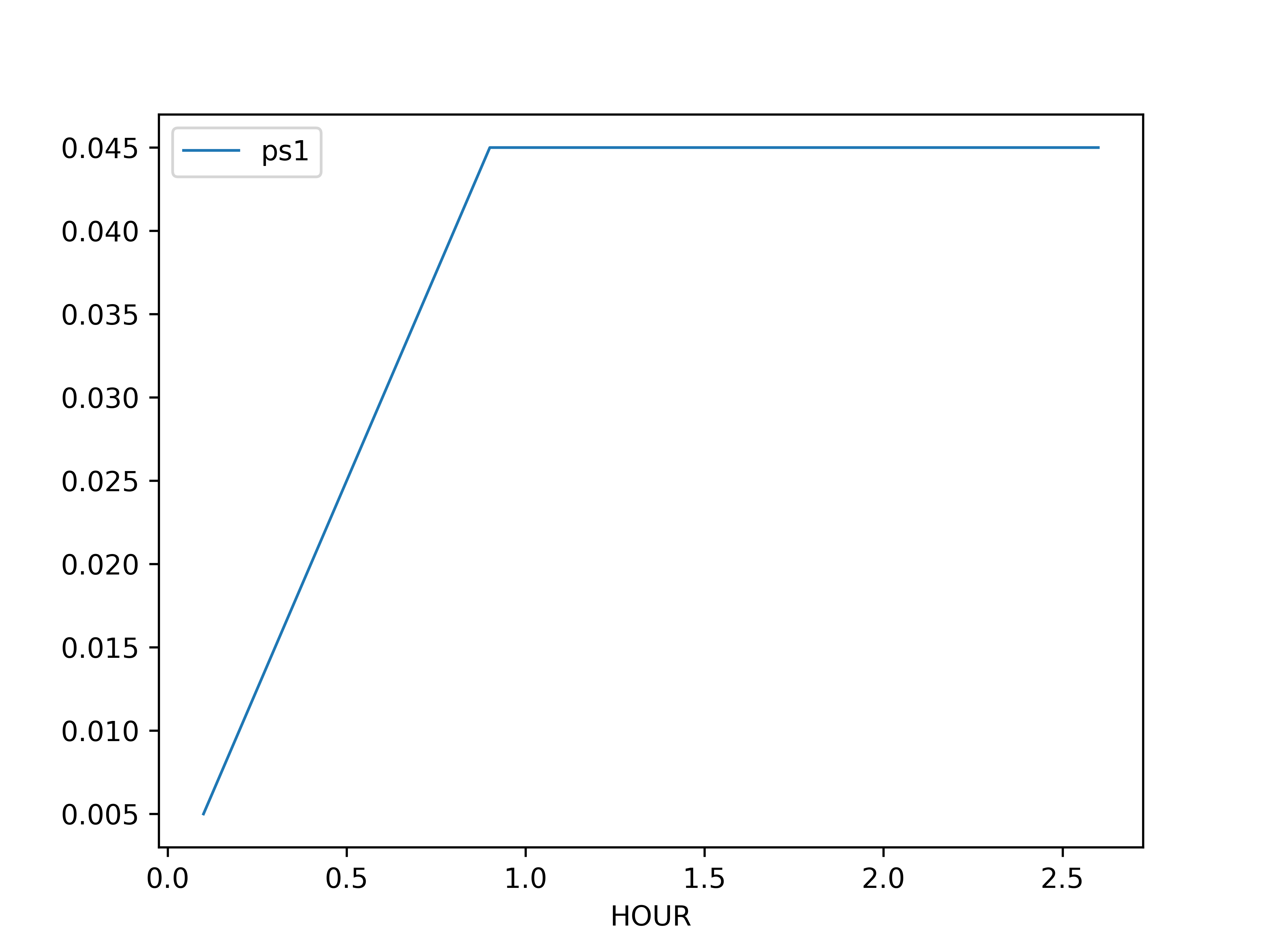
Fig. 3 ENS