Traditional power system, Monte Carlo

Here we present how to run a small Monte Carlo simulation of the behavior of the network presented in the system setup section to illustrate how RELSAD can be used.

Monte Carlo simulation

To run a Monte Carlo simulation the user must specify:

• The number of iterations, iterations

• Simulation start time, start_time

• Simulation stop time, stop_time

• Time step, time_step

• Time unit presented in results, time_unit

• A callback function, callback

• List of Monte Carlo iterations to save, save_iterations

• Saving directory for results, save_dir

• Number of processes, n_procs

sim = Simulation(power_system=ps, random_seed=0)
sim.run_monte_carlo(
    iterations=10,
    start_time=TimeStamp(
        year=2019,
        month=0,
        day=0,
        hour=0,
        minute=0,
        second=0,
    ),
    stop_time=TimeStamp(
        year=2020,
        month=0,
        day=0,
        hour=0,
        minute=0,
        second=0,
    ),
    time_step=Time(1, TimeUnit.HOUR),
    time_unit=TimeUnit.HOUR,
    callback=None,
    save_iterations=[1, 2],
    save_dir="results",
    n_procs=1,
)

The callback argument allows the user to specify events on an incremental basis. It is useful of you want to investigate how a given set of events impact the system reliability for varying repair time etc.

The results from the simulation are found in the specified save_dir. They include system reliability indices as well as bus information.

Here we plot ENS (Energy Not Supplied) for the power system:

path = os.path.join(
    "results",
    "monte_carlo",
    "ps1",
    "ENS.csv",
)

df = pd.read_csv(path, index_col=0)
fig, ax = plt.subplots()
df.hist(ax=ax)

fig.savefig(
    "ENS.png",
    dpi=600,
)

print(df.describe())

The plot should look like this:

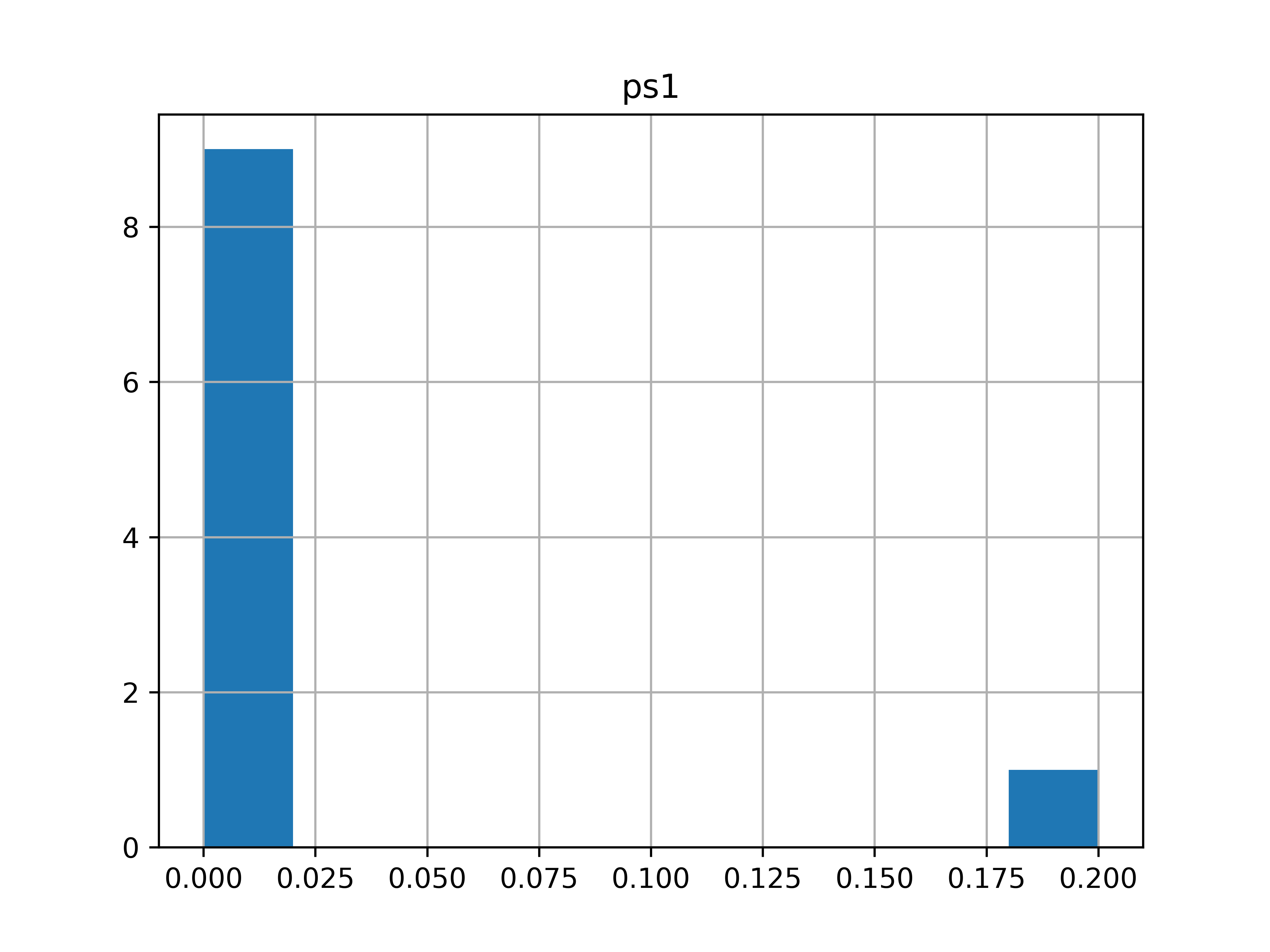
Fig. 2 ENS